LLM Inference 101

Prefill, decode, and the one number that tells you which of them is actually your bottleneck

Aug 20, 2026

Hi there 👋,

You have shipped an LLM feature. It works. Then someone asks why it costs what it costs, or why the first token takes 900ms, and you open the serving documentation.

Chunked prefill. PagedAttention. Speculative decoding. Continuous batching. GQA. Every release note announces a technique, every technique announces a speedup, and none of them tell you the thing you actually need to know: whether it solves the problem you have. So you turn on the flags a blog post recommended, watch throughput improve, and then watch your p99 get worse for reasons nobody explains.

The gap is not knowledge of the techniques. It is the layer underneath them.

You cannot pick an optimization until you know which resource is on your critical path. Most teams are tuning the one that is not.

Back in May we published ten techniques for cutting inference latency. That post was the what. This one is the why: the mechanics between your request and the text that comes back, and the arithmetic that tells you where the time is going. Read this and you will be able to open a serving paper or a vendor benchmark and identify the bottleneck being targeted without anyone explaining it to you.

No CUDA or training experience required. If you understand matrix multiplication, you are ready.

We want to introduce Dev Jadhav as the guest author on this one.

Dev Jadhav is a Staff level ML Systems Engineer specializing in LLM inference, distributed training, evaluation, AI infrastructure, and production GenAI systems.

Through MLwithDev and GitHub, he writes about the engineering behind modern AI systems, connecting research papers and emerging architectures with hands-on implementations and production trade-offs.

His open-source work includes DeepSeek from Scratch, where he explores techniques such as Multi-Head Latent Attention, Mixture-of-Experts, multi-token prediction, FP8, GRPO, knowledge distillation, and distributed training; Intelligent Routing, a Rust-based project for efficiently distributing workloads across large accelerator fleets; and SRenity, an agentic SRE platform focused on observability, anomaly detection, and AI-assisted incident response.

His broader work sits at the intersection of AI research and systems engineering, with a particular interest in understanding frontier architectures from first principles and translating them into practical, efficient, and production-ready implementation. Through MLwithDev, he shares these learnings with engineers interested in building and operating the next generation of AI systems.

The 30 second version

Generating text on a GPU splits into two execution regimes with opposite characteristics.

Prefill reads your whole prompt in parallel. Given enough prompt tokens, it does a lot of arithmetic per byte of model weight it loads, so it usually runs out of compute first.

Decode writes the answer one token at a time. At small batch it does very little arithmetic per byte loaded, so it usually runs out of memory bandwidth first.

Most serving optimizations are attacking one of those two facts. Not all of them, and the two regimes are not the only things that can be your bottleneck, which is a point I will come back to and make precise rather than hand wave.

Part 1: What actually happens between prompt and text

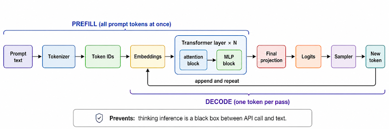
Almost every inference article starts at “prefill.” That skips the part you need in order to understand prefill. Here is the whole path.

Tokenization. Your text is split into subword units called tokens and each becomes an integer ID. For English prose a token is often a fraction of a word, roughly 0.75 words on average, but the ratio swings hard for code, for numbers, and for non-English languages. Token counts are not word counts, and your bill is in tokens.

Embedding. Each token ID indexes into a big lookup table and comes out as a vector, typically a few thousand numbers wide. This is d_model.

The transformer layers. That vector passes through a stack of identical layers (Llama 3.1 70B has 80 of them). Each layer has two blocks:

An attention block, which lets each token position pull information from other positions. This is the only place where tokens talk to each other.
An MLP block (also called the feed-forward network), which transforms each position independently. Roughly two thirds of the arithmetic in a dense model lives here, which surprises people who assume attention dominates.

Both blocks are wrapped in normalization and residual connections.

Logits. After the last layer, a final projection produces one score for every token in the vocabulary. Those scores are the logits.

Sampling. A rule picks one token from those scores. That token is appended to the sequence and the whole thing runs again for the next token.

Inside the attention block: Q, K and V

You need this to understand everything in Part 5, and most 101 articles skip it.

In each layer, every token position produces three vectors:

a query: what am I looking for?
a key: what do I offer?
a value: what do I contribute if you pick me?

Attention for a given token is: compare my query against every key from every earlier position, turn those comparison scores into weights, and take a weighted sum of the corresponding values.

Now notice the asymmetry, because it is the whole reason the next few parts exist. At step t you compute attention for token t only, so you need exactly one query, the one you just made. But you need every key and every value from positions 1 through t.

And here is the part that makes caching possible: once an earlier token has been processed through a layer, its key and value for that layer do not change just because more tokens got appended after it. They are fixed.

One query, used once and thrown away. All the keys and values, needed forever and never changing. That is why it is called the KV cache and not the QKV cache.

(This is also a very common interview question.)

How this differs from training

If your mental model is “batch of examples, forward, backward, optimizer step,” inference will feel strange until you make this contrast explicit.

Training is a compute-heavy exercise with fixed tensor shapes, no sequential dependency between examples in a batch, and enormous parallelism. Inference is a sequential loop with ragged, constantly changing shapes, where different requests are at different lengths and new ones arrive mid-flight. Training is mostly a scheduling-free arithmetic problem. Inference is mostly a scheduling problem wrapped around a bandwidth problem.

Checkpoint Q: Why can the model cache keys and values but not queries?

A: Keys and values for past positions are fixed once computed and are needed at every future step. A query is consumed immediately by the step that created it.

Part 2: Which token comes out

The sampler is the last step of every single token, so it belongs here rather than being buried nine sections later.

Greedy. Take the highest scoring token. Deterministic, tends toward repetition.
Temperature. Scale the logits before converting to probabilities. Higher flattens the distribution, lower sharpens it.
Top-k. Sample only from the k highest scoring tokens.
Top-p (nucleus). Sample from the smallest set of tokens whose probabilities sum to p. Adapts better than top-k when the model is very confident or very unsure.
Beam search. Track several candidate sequences at once. Helps some tasks, but multiplies both cache and compute per request, so it is rare in high-throughput chat serving.

Constrained decoding forces output to match a schema: valid JSON, a regex, a grammar. At each step the engine masks out tokens that would break the rules. It is cheap relative to a forward pass, though not free: grammar compilation and per-step logit masking have real, workload-dependent cost. It is the single most useful reliability feature for tool calling and data extraction.

Part 3: Prefill and decode

Everything so far described one forward pass. Now the split.

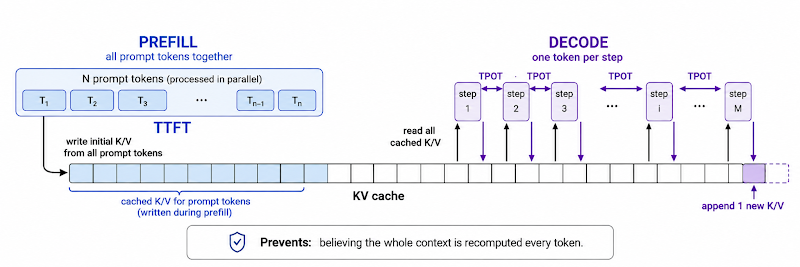
Prefill runs your entire prompt through the stack at once. All prompt positions go through the layers together, because the causal mask lets you compute them in parallel even though each attends only to earlier ones. Out comes the first token, and the keys and values for every prompt position get written into the cache. The time until you see the first character is time to first token (TTFT).

Decode then runs the loop: one new token in, its K and V appended to the cache, attention computed against the whole cache, one new token out. Repeat. The gap between words appearing is time per output token (TPOT), also called inter-token latency.

Sarathi-Serve (Agrawal et al., OSDI 2024) puts the difference cleanly: prefill iterations have high latency but saturate GPU compute because they process the prompt in parallel, whereas decode iterations have low latency and low compute utilization because each handles a single token per request.

The kitchen

One picture to carry through the rest of the article.

A chef with superhuman knife skills keeps her ingredients in a warehouse across town. Driving there and back takes 20 minutes. Chopping takes 30 seconds. If she cooks one dish per trip, her knife skills are irrelevant: she is limited by the truck. If she takes 32 orders and cooks them all from one haul, the drive amortizes and her knife skills finally matter.

The knife is the GPU’s compute. The truck is memory bandwidth. The warehouse inventory is the model weights.

One correction to the analogy before it misleads you: the truck is not only carrying shared ingredients. Every order also brings its own recipe notes, and those are not shared with anyone. That is the KV cache, it grows per user, and it does not amortize the way the weights do. Hold that thought until Part 5, because it is where the free lunch ends.

Part 4: Why the two phases have opposite bottlenecks

A GPU computes (multiplies and adds) and it moves bytes (reads weights and data from HBM, its main memory, into the compute units). Both happen at once. Whichever finishes last is your bottleneck.

The tool for telling them apart:

arithmetic intensity = (arithmetic performed) / (bytes moved from memory)
                     = FLOPs / bytes

“For every byte I drag out of memory, how much work do I get out of it?”

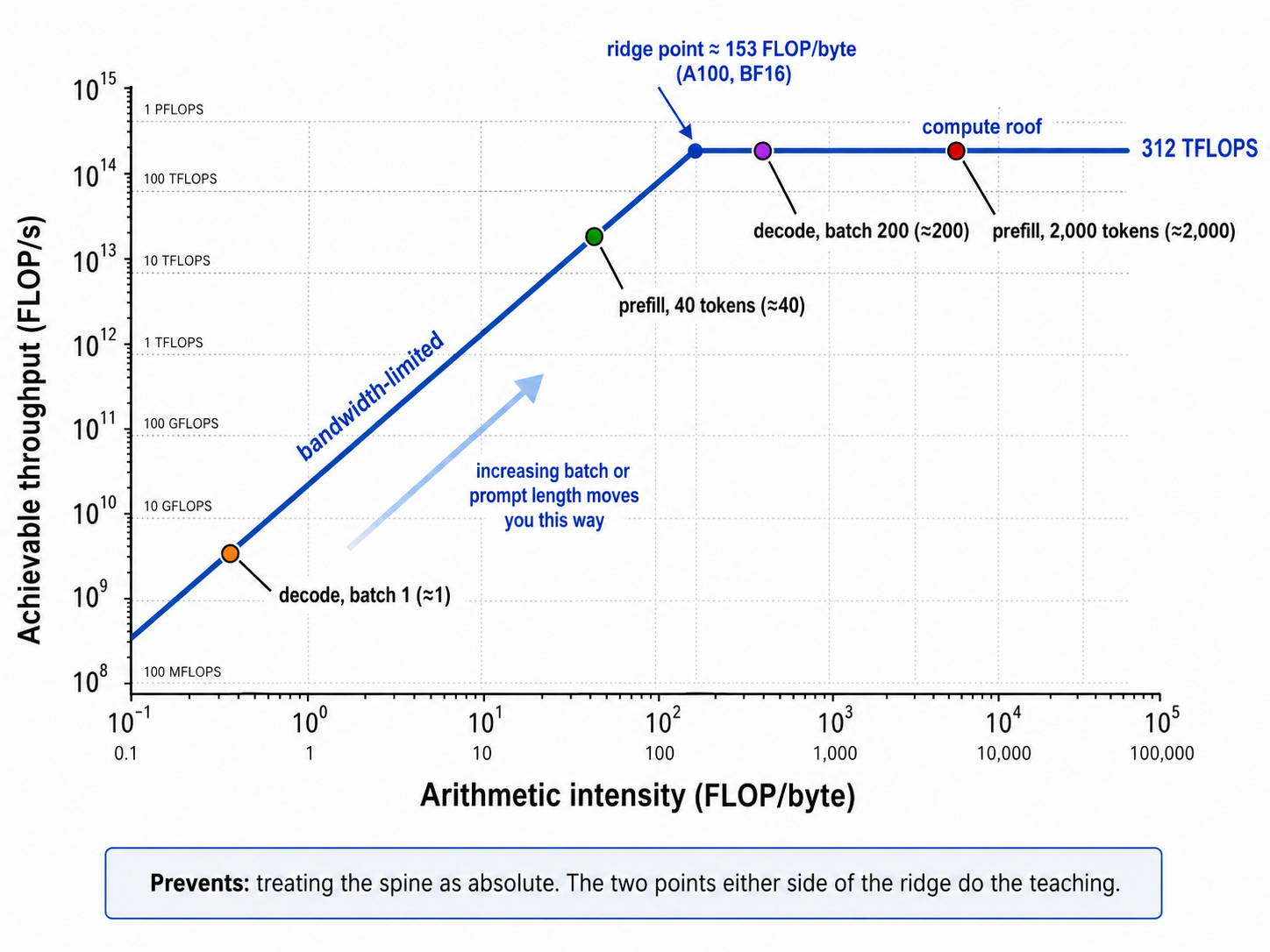
Every GPU has a break-even ratio where compute time equals memory time. It is called the ridge point. Take the A100 80GB SXM: 312 TFLOPS of BF16 tensor core compute, 2,039 GB/s of bandwidth.

ridge point = 312e12 FLOP/s / 2.039e12 byte/s = 153 FLOP per byte

Above 153 FLOP/byte you are compute-limited. Below it you are bandwidth-limited. That number is the most useful thing in this article.

Where the two phases land

The following model is deliberately simple. It counts only weight traffic for a dense, decoder-only model in BF16, and ignores KV traffic, activations, kernel inefficiency and communication. It is a lower bound on complexity and an upper bound on performance. It is still the right first model, as long as you know that is what it is.

Decode at batch 1. To emit one token, the model reads essentially every weight once. With P parameters: about 2P FLOPs (one multiply and one add per parameter, against that token’s activations) and about 2P bytes (two bytes per parameter at 16-bit).

intensity ≈ 2P FLOPs / 2P bytes = 1 FLOP per byte

One, against a ridge point of 153.

Two things worth noticing. First, the two 2s cancelling is a coincidence of BF16. At FP8 the intensity is 2, at INT4 it is 4. Quantization is partly a way of raising decode’s arithmetic intensity, which is a cleaner way to think about it than “smaller files load faster.” Second, at batch size B this becomes roughly B FLOP/byte, because you do B tokens’ worth of arithmetic per weight load.

Prefill. With T prompt tokens, the same weight load serves T tokens of arithmetic, so intensity scales with T.

The thresholds, which are what make this engineering rather than a slogan

Now run the two thresholds, because “prefill is compute-bound, decode is memory-bound” without them is a slogan.

Prefill with a 2,000 token prompt: intensity in the thousands. Compute-bound, comfortably.
Prefill with a 40 token prompt: intensity around 40, which is below 153. That prefill is bandwidth-bound. Short agentic tool-call turns and one-line chat replies live below that line constantly.
Decode at batch 200: intensity around 200, above 153. That decode is no longer purely bandwidth-bound.

So the honest version is: prefill above roughly 150 prompt tokens is compute-bound on an A100, and decode below roughly batch 150 is bandwidth-bound on an A100, for the dense linear layers. Different GPU, different threshold. Different precision, different threshold.

And there are more than two bottlenecks

Compute and bandwidth are the two you hit first on a single GPU. At production scale two more show up, and both bite hardest exactly where decode already hurts:

Communication-bound. Multi-GPU decode does an all-reduce every layer. At small batch that collective can dominate the step.
Overhead-bound. At small batch on small models, CPU-side kernel launch and scheduling cost can be a large fraction of step time. This is precisely why vLLM and TensorRT-LLM capture the decode step into CUDA graphs.

Memory capacity and scheduler queueing are also real limits, and neither is visible in an arithmetic intensity calculation.

The useful habit is not “prefill or decode.” It is: what work is happening, what bytes move, what communication happens, and which resource is actually on the critical path?

Checkpoint Q: Same model, same GPU. Why is a 2,000 token prefill compute-bound and a 40 token prefill not?

A: Intensity scales with how many tokens share one weight load. Forty tokens per load is below the A100’s 153 FLOP/byte ridge point.

Part 5: The KV cache

You already know why it exists from Part 1: keys and values for past positions are fixed and needed at every step, so we store them instead of recomputing them. Now the cost.

Deriving the size

One token, one layer, one KV head: one key vector and one value vector, each head_dim long. That is 2 × head_dim numbers.
Times the number of KV heads and the number of layers.
Times bytes per number.
That is one token. Times context length, times number of concurrent users.

KV bytes = 2 × n_layers × n_kv_heads × head_dim × seq_len × batch × bytes

It grows linearly in context length and linearly in concurrent users. Neither of those amortizes across the batch the way weights do.

Real numbers

Llama 3.1 70B: 80 layers, 64 query heads but only 8 KV heads, head_dim 128, BF16. (Eight KV heads instead of 64 is Grouped Query Attention, and it is already an 8x saving. More on that in Part 10.)

Per token, per user:

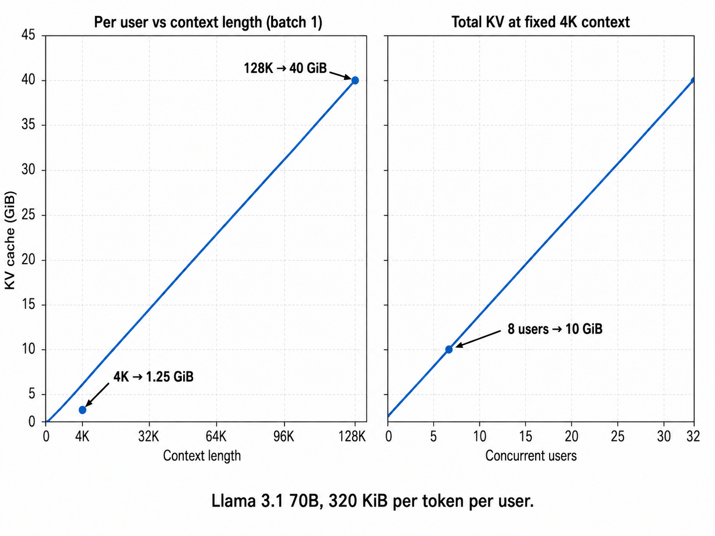
2 × 80 × 8 × 128 × 2 bytes = 327,680 bytes = 320 KiB per token

320 KiB per token. Remember that one. Now:

1 user, 4K context : 1.25 GiB KV cache
8 users, 4K context: 10 GiB KV cache
1 user, 128K context: 40 GiB KV cache
8 users, 128K context: 320 GiB KV cache

The weights of this model in BF16 are about 140 GB, and they are a fixed cost. The cache is not. Once the weights are resident, the remaining memory budget is what determines how much concurrency and context length your server can actually support.

The second problem

Each decode step’s new query attends to the stored keys and values for all previous positions, so KV traffic grows with the number of attended tokens. That means generation gets slower as the conversation gets longer, on top of using more memory. The cache is both the thing filling your GPU and part of what you are bandwidth-limited on.

(Sliding-window and hybrid attention architectures bound this deliberately, which is exactly why they exist.)

Checkpoint Q: Weights amortize beautifully across a batch. Why does the KV cache not?

A: All users share one copy of the weights. Every user has their own cache, so cache bytes scale with batch while weight bytes do not.

Part 6: Where GPU memory actually goes

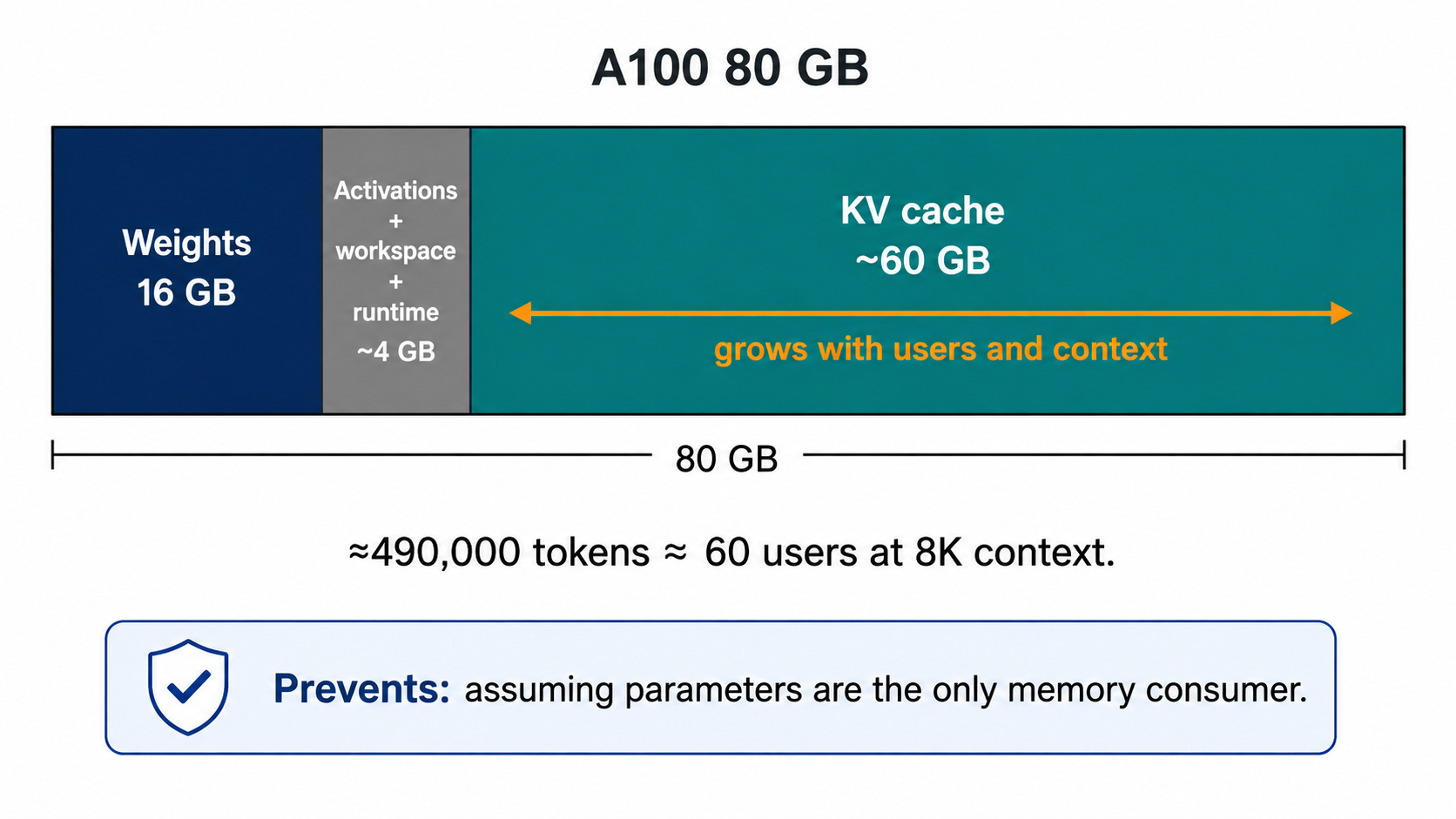
“The model fits” is not the same as “the model serves.” Four things compete:

Weights. Parameters times bytes per parameter. A 7B model in BF16 is about 14 GB. Llama 3.1 70B is about 140 GB.
KV cache. Everything in Part 5. This is the part that grows with load.
Activations and workspace. Intermediate tensors for the tokens currently in flight, plus scratch buffers for the kernels. Scales with batch and with prefill chunk size.
Runtime overhead. CUDA context, framework allocations, communication library buffers. A few gigabytes before you serve a single request.

Worked example. Llama 3.1 8B on one A100 80GB (32 layers, 8 KV heads, head_dim 128, so 128 KiB per token of cache):

  80 GB total
- 16 GB weights
- ~4 GB activations, workspace and runtime overhead
= ~60 GB available for KV cache

60 GB / 128 KiB per token ≈ 490,000 tokens of aggregate cache
                          ≈ 60 concurrent users at 8K context each

That final number is your actual serving capacity, and you cannot get to it from the parameter count alone.

Part 7: Measuring it

The metrics

TTFT. Queue wait plus tokenization plus prefill. Note the first term. Under load, TTFT is dominated by queueing, which makes it a scheduling property rather than a GPU property.
TPOT / ITL. Steady-state per-token generation time.
End-to-end latency. TTFT + (N_out − 1) × TPOT, since TTFT already covers the first token.
Throughput. Aggregate output tokens per second across all users. Also requests per second.
Tokens per second per user. A completely different number from throughput.
p50, p95, p99. Averages hide the problem. Continuous batching and large batches typically improve p50 while worsening p99, because a long prefill blocking the queue is a tail phenomenon. p99 TTFT is the number that gets people paged.
Goodput. Throughput that meets your latency targets. Raw throughput at unacceptable latency is worthless, which is why production systems cap batch size and shed load rather than accepting everything.

A worked example

Prompt 1,000 tokens, output 100 tokens, TTFT 400 ms, TPOT 25 ms.

E2E = 400 ms + 99 × 25 ms = 2,875 ms ≈ 2.9 s
Per-user generation rate = 1 / 0.025 = 40 tokens/sec

Now double your throughput by doubling batch size, and suppose TPOT rises to 35 ms:

E2E = 400 ms + 99 × 35 ms = 3,865 ms ≈ 3.9 s

You served twice as many people and made every one of them wait 34% longer. That trade is the job. There is no configuration that wins both.

Ceilings versus measurements

Every number I computed in Part 4 and Part 6 is a ceiling. It assumes you hit 100% of the GPU’s rated bandwidth. You will not.

Real serving stacks land at roughly 60 to 80% memory bandwidth utilization (MBU). So the batch-1 ceiling of 127 tokens/sec for Llama 3.1 8B on an A100 (16 GB / 2,039 GB/s = 7.85 ms per token) corresponds to something like 80 to 100 tokens/sec in practice. The gap is kernel launch overhead, non-weight traffic, and imperfect kernels.

Here is why the model is still worth trusting, and this is the best demonstration I can give you that it works. The AWQ paper reports Llama-2-7B on an RTX 4090 going from 52 to 194 tokens/sec with INT4 weight quantization. Check it against the roofline yourself. The 4090 has 1,008 GB/s of bandwidth:

FP16: 13.5 GB of weights → 1008 / 13.5 = 74.7 tok/s ceiling
      reported 52  → 70% MBU

INT4: ~3.5 GB of weights → 1008 / 3.5  = 288 tok/s ceiling
      reported 194 → 67% MBU

Both land at about 70% MBU. The reported numbers are internally consistent with a simple bandwidth model, and the speedup is almost exactly the weight-size ratio. You just validated a vendor benchmark with arithmetic you learned twenty minutes ago. That is what the mental model is for.

Checkpoint Q: Your dashboard shows throughput up 60% after a config change, and users are complaining. What do you look at?

A: p95 and p99 TTFT and TPOT. You most likely traded tail latency for aggregate throughput.

Part 8: Batching

Decode at batch 1 leaves most of the compute idle. Batching fills it: load each weight matrix once, then push many users’ current tokens through the same matrix multiply.

The ceiling, and then the reality

Llama 3.1 8B on an A100. At batch 1, a decode step is bounded by streaming 16 GB of weights at 2,039 GB/s, so 7.85 ms per token, so 127 tokens/sec. At batch 32 the weights are still read once, so if weight streaming were the only cost, you would get 32 tokens per 7.85 ms, or about 4,050 tokens/sec.

That is an upper bound, not a forecast. Real gain is closer to 20 to 25x, for reasons you can now name:

KV cache reads scale with batch and do not amortize (Part 5).
Attention kernel work grows with batch and context.
Step time typically rises 10 to 30% at batch 32.
You are at 60 to 80% MBU, not 100%.

Twenty times is still an enormous win. State it as twenty rather than thirty-two and you will be believed.

Three kinds of batching

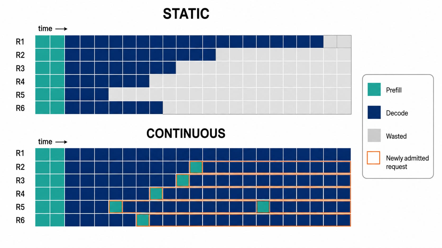
Static. Fix a group, run until the last one finishes. Short requests idle behind long ones.
Dynamic. Collect arrivals for a short window, then launch. Better utilization, still finishes as a group. This is what a classic Triton dynamic batcher does.
Continuous (in-flight). Re-decide batch membership every token step. Finished requests leave immediately, waiting requests join immediately. Introduced as iteration-level scheduling in the Orca paper (OSDI 2022).

Anyscale’s benchmark of continuous batching plus vLLM’s memory management reported up to 23x higher throughput than naive batching, on OPT-13B on one A100 40GB. That is one workload on one model on one card, and the shape of the result generalizes better than the number does.

[FIGURE 6: static vs continuous batching]

And the tension it creates

Bigger batch means more work per step, so per-user latency can degrade. Worse, admitting a long compute-heavy prefill into the batch stalls everyone’s decode, which is a tail-latency event.

The standard fix is chunked prefill: split a long prefill into pieces and interleave them with ongoing decodes, so new requests join without pausing active ones. Sarathi-Serve reported throughput gains within latency targets of up to 2.6x for Mistral-7B on one A100 and up to 5.6x for Falcon-180B on eight A100s with pipeline parallelism. Prefill-interleaved scheduling of this kind is now widely used in production engines, and vLLM enables chunked prefill by default where it can.

Part 9: What a production inference server actually looks like

The GPU is one box out of seven. This is the diagram that connects “what a transformer does” to “why vLLM exists.”

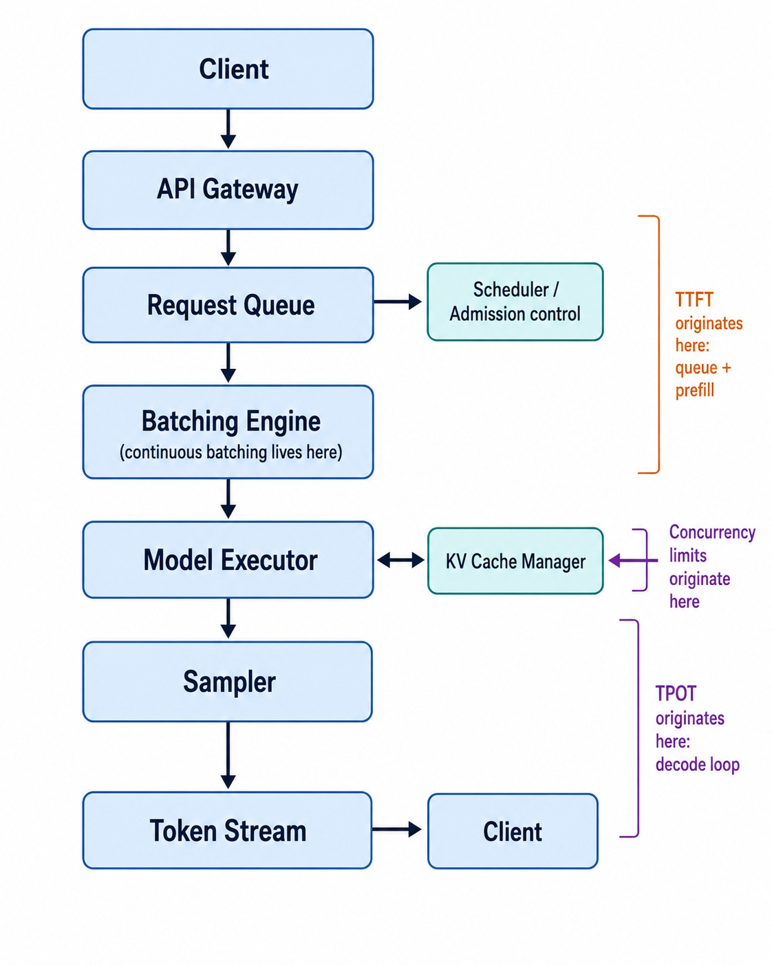
Where each metric comes from:

Queue plus prefill → TTFT
Decode iterations → TPOT
Scheduler and batching engine → throughput and goodput
KV cache manager → concurrency and context limits
GPU workers → compute, bandwidth and communication limits

The engines. vLLM is the open source default and where most people should start. SGLang shines when requests share structure, such as agents and RAG, because it aggressively reuses cached prompt prefixes. TensorRT-LLM is NVIDIA’s compiled engine, highly optimized for NVIDIA hardware, at the cost of a compilation step and real tuning effort; whether it beats the alternatives depends on your model, hardware and workload. llama.cpp is the right answer for local and edge.

Part 10: The optimization map

You now have enough to place every technique you will meet. Each row is an answer to “what resource does this free up?”

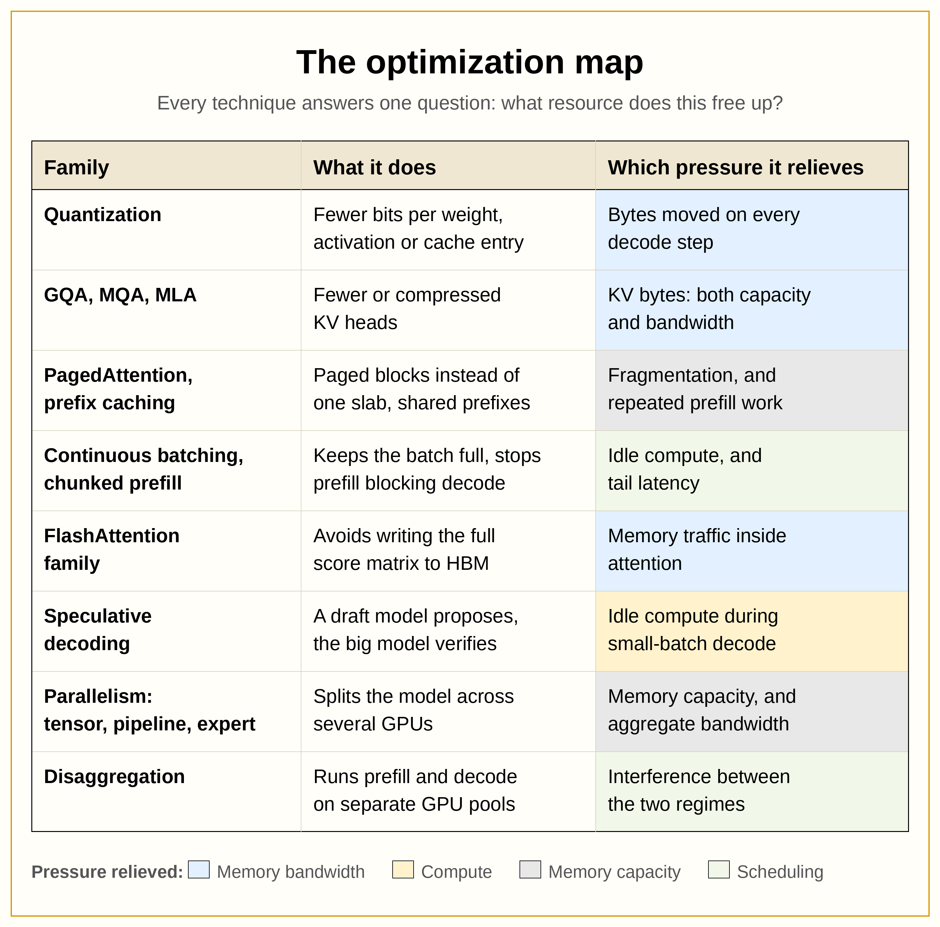
The one that catches everyone: more GPUs does not mean faster tokens per user. Pipeline and expert parallelism scale system throughput. Only tensor parallelism improves single-user latency, and only until the per-layer collective starts dominating.

Part 11: Misconceptions worth carrying away

“Bigger batch always helps.” It helps until you approach the ridge point or run out of KV capacity. Past that, per-user latency degrades for nothing.

“Quantization always speeds things up.” It depends on what you quantized and what your bottleneck is. Weight-only quantization targets bandwidth. And INT4 only pays off if dequantization is fused into the compute kernel; if your library dequantizes to 16-bit in a separate pass, you moved the full-size bytes anyway.

“More GPUs means faster tokens per user.” See above.

“Throughput and latency can both be optimized for free.” They trade against each other directly. That tension is why chunked prefill, goodput and admission control exist.

“The weights are what fill my GPU.” The weights are a fixed cost. The KV cache is the one that grows with your traffic, and it is usually what caps you.

“Prefill is compute-bound and decode is memory-bound.” True as a first-order default at typical prompt lengths and small batch. Not true for short prompts, not true at very large batch, and not the whole story once communication and per-step overhead enter the picture.

The takeaway

Prefill and decode create very different workloads. Prefill exposes a lot of parallelism and reuses each loaded weight across many tokens. Small-batch decode exposes very little and therefore tends to be bandwidth-sensitive. To understand any inference optimization, ask what computation it avoids, what bytes it avoids moving, what state it consumes, and which resource is actually on the critical path.

That last clause is the part that keeps working after the article ends. The critical path is usually compute or bandwidth. Sometimes it is the interconnect, the scheduler, or the CPU launching your kernels. Arithmetic intensity tells you about the first two, and you now know how to compute it.

Next time you read a paper announcing a new serving technique, do not start with the mechanism. Start by asking which resource it frees. The mechanism will make sense immediately afterward.

Glossary

Arithmetic intensity. Arithmetic performed per byte moved from memory. Compare against the ridge point.

Continuous batching. Re-forming the batch every token step so requests join and leave immediately.

Decode. The phase generating output one token at a time.

Goodput. Throughput that meets your latency targets.

HBM. The GPU’s main memory. Large, and far slower than on-chip SRAM.

KV cache. Stored key and value vectors for past positions. Grows linearly with context and with concurrent users.

Logits. The per-vocabulary-token scores produced after the final layer.

MBU. Memory bandwidth utilization. Fraction of rated bandwidth actually achieved. Real systems land around 60 to 80%.

PagedAttention. Operating-system-style paging of the KV cache into small non-contiguous blocks.

Prefill. The phase reading the whole prompt in parallel and producing the first token.

Ridge point. The arithmetic intensity at which compute time equals memory time on a given GPU. About 153 FLOP/byte for an A100 at BF16.

TTFT / TPOT. Time to first token, time per output token.

A guest post by

MLwithDev

Staff ML Systems Engineer exploring how modern AI works in production. Writing about LLM inference, AI infrastructure, evaluation, distributed systems, agents, and frontier-model engineering through first principles, trade-offs, and implementation.

Immanuel Santosh

19h

The prefill vs decode distinction is exactly what Indian startups miss when budgeting AI infrastructure.

Most founders I advise budget for GPU cost alone, ignoring that decode-bound workloads need bandwidth optimization, not just compute scaling.

For cost-sensitive teams, understanding this split is the first step to deciding whether to optimize inference or simply outsource it.

Discussion about this post

Ready for more?