Reinforcement Learning in Finance: From Bellman Equations to Deep Q-Networks

Real-world Reinforcement Learning project: Part 1

Hey there 👋

Welcome to Part 1 of a new mini-series on Reinforcement Learning in Finance, with a special focus on pricing options.

This series is based on one of my projects from 2021 and still very valid, and rewritten in a way that you can actually read on a Sunday afternoon without needing three coffees and a PhD in stochastic calculus 😅

When I started this project, I knew almost nothing about Reinforcement Learning or Option Pricing in Finance. I didn’t walk in as an expert, I walked in with a problem I didn’t fully understand and a huge learning curve in front of me.

By the end of it, that “scary” problem turned into:

• A working RL solution for a real quant finance task

• A PhD position offer

• And great job opportunities that opened up because I could show I’d tackled something non-trivial, end-to-end

That’s exactly what I want this series to give you:

Not just “RL as in AlphaGo”

Not just Titanic datasets, toy regressions, or yet another RAG / agentic AI demo

…but Reinforcement Learning on a real financial problem:

How do you learn an optimal exercise strategy for an option from scratch?

If you stick with this series, you’ll see how we go:

• From core Reinforcement Learning concepts

• To understanding what are options in finance

• To designing and training deep RL agents that actually price these options

My goal is simple:

By the end, you should look at RL and think,

“I can use this on serious problems, not just classroom examples.”

Alright, let’s dive right in.

---

Why Reinforcement Learning in Finance?

Traditional quant finance is full of beautiful closed-form formulas and elegant Partial Differential Equations (PDEs).

But reality is messy:

• Financial Markets are noisy and non-stationary

• You have constraints (capital, risk limits, liquidity)

• You make sequences of decisions over time, not just one-off predictions

That’s exactly the world Reinforcement Learning (RL) was built for:

An agent interacting with an environment, taking actions over time, and learning to maximise long-term reward.

In finance, that could mean:

• When to exercise an option

• How to dynamically hedge a portfolio

• How to allocate capital across multiple instruments

In this series, we’ll focus on one concrete problem:

Learning optimal exercise strategies for American options using deep RL.

But before we model American options as an RL problem, we need a clean mental model of RL itself.

✅ That’s today’s job.

---

Where RL fits in the ML Landscape

Let’s quickly place RL in the bigger Machine Learning universe:

• Supervised learning

  • You get labelled data: (x, y) pairs.

  • Example: predict tomorrow’s return from historical features.

  • Objective: minimise prediction error (MSE, cross-entropy, etc).

• Unsupervised learning

  • No labels. You discover structure.

  • Example: clustering similar stocks, PCA on yield curves.

• Semi-supervised / self-supervised

  • Mix of labelled + unlabelled data, or clever pretext tasks.

• Reinforcement learning

  • No fixed dataset of “correct answers”.

  • An agent interacts with an environment:

    • Observes a state

    • Takes an action

    • Receives a reward

  • Objective: maximise cumulative reward over time.

In RL, “ground truth” is not handed to you.

The agent discovers a good strategy by trial and error.

This is exactly like a trader learning a strategy by simulating trading in a market model: they try actions, see Profit & Loss outcomes, and adjust.

Note: Here the agent is not the LLM AI agent that we see and talk about almost everyday 😉

---

Quick Detour: What Are Options?

Before we jump into Reinforcement Learning, let’s quickly understand the financial instrument at the heart of this series.

An option is a simple but powerful contract, it gives you the right (not the obligation) to buy or sell an asset at a fixed price (called the strike price) within a certain time period.

Think of it as a bet on future prices:
you pay a small premium today for the possibility of a big payoff later; if you are right about where the market goes you profit from this transaction. If the market does not go according to what you had predicted, you will choose to NOT exercise your right and your option will expire worthless i.e., your loss will only be the “Premium” you paid to purchase this “option” contract. In this series we want to use Reinforcement Learning to price this “premium” on options.

Note: there are two types of options, American vs. European which will be exalted in the second part of this Blog series.

Options are how some investors made legendary fortunes.

Remember Dr. Michael Burry from The Big Short?

He used options to bet against the U.S. housing market, and walked away with hundreds of millions when his prediction came true.

They’re incredibly powerful, but also tricky to value and that’s exactly the challenge we will tackle in this series.

---

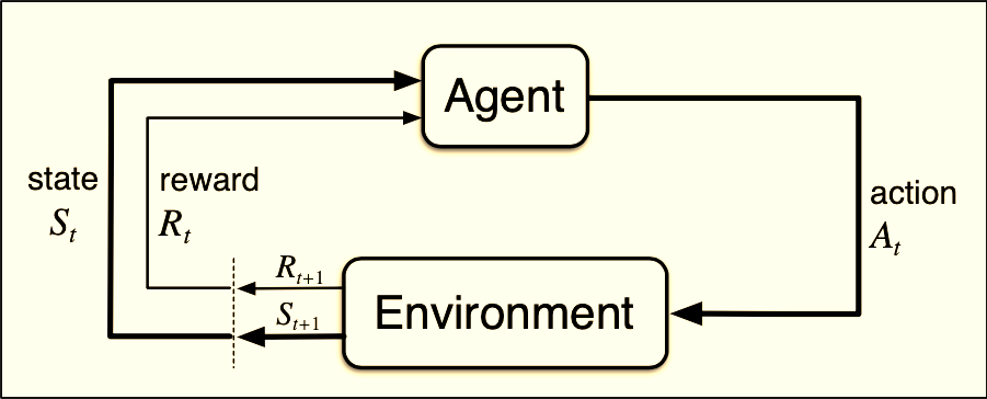
The Agent-Environment Loop

The core of Reinforcement Learning is a simple loop:

1. The agent observes the current state

2. It chooses an action

3. The environment responds with:

   • a new state

   • a reward

Repeat this thousands or millions of times.

In a financial-trading mental model:

• State = information you have now

  • e.g. current price, time, volatility estimate, portfolio holdings

• Action = what you do now

  • buy, sell, hold, exercise the option, rebalance the hedge, etc.

• Reward = what you “get” at this step

  • P&L increment, utility, negative transaction cost, etc.

• Episode = one complete scenario / path

  • e.g. full price path from trade initiation to maturity.

In our option example later:

• State = (current underlying price, time to maturity, maybe more features)

• Action = {exercise now, hold}

• Reward = zero most of the time, then payoff when you exercise or at maturity

Already sounds like an RL problem, right? Hold that thought for Part 2. 😉

---

Thinking Like an Investor: Rewards Over Time

In finance and RL, we don’t judge performance by one lucky trade.

We care about the total journey, the stream of outcomes that add up to success (or loss). That’s exactly how RL thinks. Instead of focusing on one reward, it tracks the cumulative return:

\(\begin{align} G_t &= R_{t+1} + \gamma R_{t+2} + \gamma^2 R_{t+3} + \dots \\[1em] R_t &= \text{reward at time } t \\ \gamma &\in [0, 1) \quad \text{discount factor} \end{align}\)

If you’re from finance, γ (gamma) should feel familiar:

• It plays the same conceptual role as a discount factor in present value:

• “A euro today is worth more than a euro tomorrow.”

You can think of γ like a “patience” parameter:

• γ close to 0 → impatient agent

  • Cares mostly about immediate reward

  • “Give me P&L now, I don’t trust the future.”

• γ close to 1 → patient / far-sighted agent

  • Cares about long horizons

  • “I’m okay sacrificing a bit today if it improves long-run payoff.”

A tiny numeric intuition:

If γ = 0.9, then:

• 1 unit of reward now = 1

• 1 unit of reward one step later ≈ 0.9

• 1 unit of reward two steps later ≈ 0.81

So future rewards still matter, just slightly less. For options, this is crucial:

• You don’t want an agent that exercises as soon as the payoff is positive

• It should weigh:

“If I wait, I might get a better payoff later - is it worth it after discounting?”

γ controls exactly this trade-off between:

• Exercise now (take the sure payoff), and

• Wait (keep the option alive and see what future prices bring).

---

Value Functions: Measuring “How Good” a Situation Is?

When you’re trading or making decisions, you always ask:

“If I’m here right now, how good is this position?”

RL formalises that same intuition with value functions.

State-value function

\( V^\pi(s)\)

This answers:

“If I keep following my current strategy from this state, what return can I expect overall?”

In plain words:

“If the price is $100 and 20 days remain, how valuable is this position if I continue with my current policy?”

---

Action-value function

\(Q^\pi(s, a)\)

This goes one step deeper:

“If I take this action right now, how good does that make my future?”

Think of it like asking two questions at each node of a pricing tree:

• If I exercise now, what’s my payoff?

• If I hold, what could I gain later?

That’s your Q-function.

In our option case, we are literally learning:

• Q(state, exercise) vs

• Q(state, hold)

and then simply choosing whichever has the higher Q-value, that becomes the learned exercise rule.

Pretty cool, right? The agent is basically rediscovering optimal exercise boundaries on its own.

---

Markov Decision Processes (MDPs):
Turning Finance into Decisions

To make all this concrete, RL wraps problems into what’s called a Markov Decision Process (MDP). Don’t let the name scare you.

It just means:

“Tomorrow depends only on what I know and do today, not on the entire past.”

Formally, we describe an MDP with:

• S - the set of possible states (like price & time)

• A - the actions (exercise or hold)

• P(s’|s,a) - how the world moves from one state to another

• R(s,a) - the reward you get for each action

• γ - your discount factor from earlier

In option pricing, that assumption fits perfectly.

If your state includes the current price and time to maturity, and the underlying follows Geometric Brownian Motion (GBM), then the next state depends only on those two.

So our environment for options is elegantly simple:

\(s_t = (S_t, t)\)

Every decision the agent makes depends on just that snapshot, not on yesterday’s full path. This is what allows RL to learn efficiently and generalise.

---

Bellman Equations: The Logic of Looking Ahead

The Bellman equation is the backbone of RL.

Here’s the golden insight behind almost all RL algorithms:

“The value of being in a situation = what you get now + what you expect to get later.”

That’s the Bellman equation in plain language.

Mathematically, for a given strategy pi:

\(V^\pi(s) = \mathbb{E}[R_{t+1} + \gamma V^\pi(S_{t+1}) \mid S_t = s]\)

It’s just a mathematical recursive version of:

“Today’s worth = today’s reward + discounted value of tomorrow.”

And for the optimal strategy, we simply take the max over all actions. You don’t need to memorise formulas, just remember this mental model:

RL algorithms keep tweaking their estimates of value until they satisfy this relationship. If you’ve ever used a binomial tree to price an option, this will click immediately:

At each node, you calculate:

“Value = discounted expected value of next step”

“For options: take the max between continuing and exercising.”

That’s literally the Bellman equation at work. Classical methods solve it with backward induction. RL learns it through experience, by simulating millions of price paths until the recursion naturally holds. So, when we train an RL agent for options, what it’s really doing is:

Learning to perform backward induction without us hardcoding the math.

And that’s the moment where finance meets AI beautifully.

---

A Map of RL Methods

RL is a big zoo of algorithms. Let’s organise it along a few important components that actually matter for us.

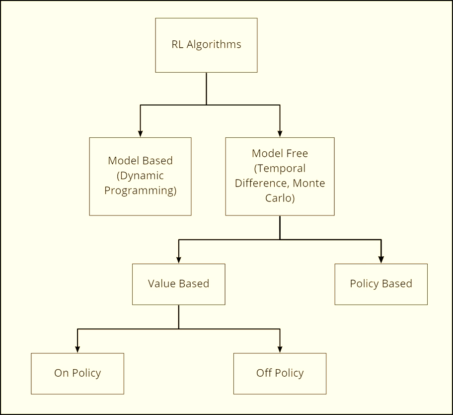
1. Model-based vs Model-free

Model-based RL

A model-based agent tries to understand how the world works before acting.
It learns (or is given) a model of how actions change the environment, like having a mini “mental simulator” of the market.

It can then plan ahead:

“If I sell now, the price might move this way; if I hold, this might happen instead.”

Model-free RL

• You don’t try to estimate the full dynamics.

• You directly learn value functions or policies from interactions.

• This is what we will use for options.

A model-free agent skips the “world modeling” part, it learns purely from experience.
It doesn’t try to predict what the market will do, it just keeps trying things, seeing rewards, and adjusting.

It’s like a trader who learns by doing:

“Whenever I exercised early, I lost potential upside, maybe waiting works better.”

This trial-and-error style is more data-hungry but often more flexible when the world is too complex to model.

Model-free RL can be simpler and more flexible than analytic solutions, especially in high dimensions.

---

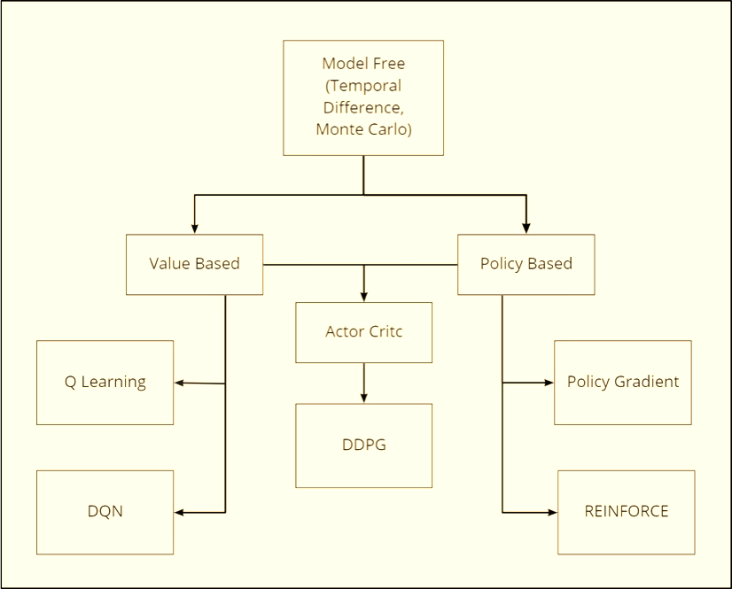
2. Value-based vs Policy-based vs Actor-Critic

Value-based methods

• Learn a value function V(s) or Q(s,a).

• The policy is implicit: pick the action with highest Q-value.

• Example: Q-learning, Deep Q-Networks (DQN).

This is a very natural fit for discrete actions like:

• exercise vs hold,

• buy vs sell vs hold.

Policy-based methods

• Learn the policy directly

• No explicit value function; you optimise parameters θ with gradient methods.

This is great for:

• Continuous action spaces (position sizes, continuous hedging ratio)

• Stochastic policies where exploration is baked in

Actor-Critic methods

• Combine both:

  • Actor: the policy

  • Critic: value function V_w(s) or Q_w(s,a)

• The critic tells the actor how good its actions were.

We won’t go deep into actor–critic in this series, but it’s the workhorse behind many advanced RL algorithms (A2C, PPO, etc.), including those used in trading and portfolio optimisation.

---

3. Monte Carlo vs Temporal Difference (TD)

Monte Carlo methods

• Learn from complete episodes.

• You wait until the end, observe the full return, and then update.

• Example: basic policy gradient (REINFORCE).

Pros: Simple, unbiased estimates of return.

Cons: High variance, slow learning, need full episodes.

Temporal Difference (TD) methods

• Learn step-by-step: bootstrap from your current estimate of value.

• Example: TD(0), Q-learning, DQN.

Pros: More sample-efficient, work in continuing tasks.

Cons: Introduce bias, need careful tuning and stabilisation.

In our option experiments:

• DQN is a model-free, value-based, off-policy TD method

• REINFORCE is a policy-based Monte Carlo method.

We’ll see in Part 3 how this difference shows up in pricing performance and stability.

---

4. On-policy vs Off-policy

On-policy RL

• You learn about the policy that is currently generating the data.

• Example: SARSA, many actor–critic methods.

Off-policy RL

• You learn about one policy while following another.

• Example: Q-learning, DQN.

In practice:

• DQN learns a greedy policy from experiences generated by an ε-greedy policy.

• That off-policy nature gives it flexibility and sample efficiency.

This distinction matters less in our option setup (because we control the simulator), but it’s crucial in real-world trading where you may reuse historical trajectories collected under different strategies.

---

Key Algorithms We’ll Use (High-Level)

Let’s briefly introduce the two main characters of Part 3: Q-learning / DQN and REINFORCE. (We will dive deeper in the next chapters.)

Q-Learning (Tabular)

Conceptually, Q-learning updates Q-values like this:

\(Q(s, a) \leftarrow Q(s, a) + \alpha \big( r + \gamma \max_{a’} Q(s’, a’) - Q(s, a) \big)\)

Intuition:

“Adjust my estimate of Q(s, a) towards: reward + discounted best future Q.”

Tabular Q-learning works when State and action spaces are small and discrete. Clearly not true for continuous prices in finance. So we need function approximation.

---

Deep Q-Networks (DQN)

DQN replaces the Q-table with a neural network:

\(Q_\theta(s, a)\)

Two crucial tricks make this stable:

1. Experience replay

   • Store transitions (s, a, r, s’) in a replay buffer.

   • Sample random minibatches to break correlation and improve stability.

2. Target network

   • Maintain a separate network for the target in the TD update.

   • Update it slowly to avoid chasing a moving target.

In our option setup:

• Input to the network: state features (e.g. normalised price, time step)

• Output: Q-values for each action {exercise, hold}

• Policy: pick action with highest Q-value (ε-greedy during training, greedy at evaluation).

---

Policy Gradient / REINFORCE

Instead of approximating Q, you directly parameterise the policy:

\(\pi_\theta(a|s)\)

You then push θ in the direction that increases expected return:

\(\nabla_\theta J(\theta) \approx \sum_t \nabla_\theta \log \pi_\theta(a_t|s_t) G_t\)

In words:

“Increase the probability of actions that led to high returns, decrease the probability of actions that led to poor returns.”

REINFORCE is:

• Simple to implement,

• But can have high variance and be unstable, especially if rewards are sparse.

You’ll see this trade-off clearly when we compare it to DQN for pricing.

---

Real-World RL: Why It’s Powerful and Painful

Before we unleash Reinforcement Learning on options, we need a sober view of its limitations.

Common pain points:

• Sample inefficiency

  RL often needs millions of interactions. In finance, real data is limited, so we rely on simulators, which might be misspecified.

• Instability & sensitivity

  Small changes in hyperparameters can completely break learning.

• Exploration vs risk

  In games, the agent can safely “try random things”.

  In markets, random exploration = real money at risk.

• Interpretability

  Deep RL policies are often black-box.

  That’s uncomfortable for risk managers, regulators, and often… you.

• Deployment gap

  What works in a simulated Geometric Brownian Motion (GBM) world may behave very differently in live, non-stationary markets.

For our option project:

• We stay in a controlled, simulated world (Black-Scholes, SABR).

• That lets us focus on:

  • Can Reinforcement Learning recover correct prices under known assumptions?

  • What are the trade-offs between different RL algorithms?

Once we understand that, we can have an honest conversation about when Reinforcement Learning is worth the complexity in real trading/hedging.

---

Putting It Together: Why This Matters for American Options

Let’s connect the dots:

• American options are about timing:

  Exercise now vs hold at each point in time.

• That’s a sequential decision problem with uncertainty in future prices.

• Reinforcement Learning is all about:

  • states (price, time),

  • actions (exercise/hold),

  • rewards (option payoff),

  • and policies that maximise expected discounted payoff.

In other words:

American option pricing = an optimal stopping problem = a perfect playground for RL.

In Part 2, we will:

• Start from standard option pricing intuition (European vs American)

• Show how American options can be framed as an optimal stopping problem

• Turn that into an explicit RL environment:

  • what is the state?

  • what are the actions?

  • how do we design the reward?

  • how do we simulate the environment (GBM, SABR)?

Then in Part 3, we will go all in on:

• Building the environment in code

• Designing and training DQN & REINFORCE agents

• Comparing RL prices to binomial / Black-Scholes benchmarks

• What worked, what broke, and what I would do differently today

---

What you should take away from Part 1

If you skimmed everything, here’s the cheat sheet:

• Reinforcement Learning (RL) is about learning from interaction, not labelled datasets.

• The core elements: state, action, reward, policy, value functions, return, γ.

• Markov Decision Processes (MDPs) + Bellman equations give the mathematical backbone.

• There are different families of RL methods:

  • model-based vs model-free

  • value-based (Q-learning, DQN) vs policy-based (REINFORCE) vs actor–critic

  • Monte Carlo vs Temporal Difference

  • on-policy vs off-policy

• Deep RL (like DQN) lets us handle continuous state spaces like asset prices.

• RL is powerful but fragile, and needs careful design, especially in finance.

  ---

Follow Along

We hope you enjoyed this learning journey.

In the next post, we will apply this toolbox to American options:

Take a very “quant finance” problem and show exactly how it becomes an RL problem.

If you want to follow along the whole series (and get access to the implementation deep dive), make sure you’re subscribed, the fun part is coming next. 💚

Remember there are problems beyond AI Agents, RAG and LLMs!

Let’s continue learning and building! 💪